Categories
Data Engineering Datawarehouse

Navigating the Data Seas: Unraveling the Landscape of Data Architectures

In the ever-evolving landscape of data management, organizations wrestle with an array of architectural patterns to make sense of the vast ocean of information. Let’s embark on a journey through four key paradigms: Data Warehouse, Data Lake, Data Lakehouse, and the decentralized marvel known as Data Mesh.

Data Warehouse: The Backbone of Structured Insights

At the core of every data-driven enterprise stands the Data Warehouse, a structured backbone that has long been a cornerstone for analytical prowess. This architectural marvel is akin to a meticulously organized library, where each piece of structured data is neatly cataloged and readily accessible.

Key Features:

  • Centralization: Acting as a centralized repository, Data Warehouses integrate structured data from diverse sources, providing a unified view.
  • Schema-on-Write: Data is structured and organized before being loaded through ETL processes, ensuring a consistent and reliable foundation.
  • SQL Dominance: Powered by SQL queries, Data Warehouses excel in supporting business intelligence (BI) and reporting applications, generating insightful reports.

Data Lake: The Uncharted Reservoir of Possibilities

In contrast to the structured rigidity of a Data Warehouse is the uncharted wilderness of a Data Lake. Imagine a vast reservoir collecting data in its raw, unstructured, or semi-structured form. Data Lakes offer unparalleled flexibility, accommodating a diverse range of data formats.

Key Features:

  • Versatility: Data Lakes embrace a multitude of data types, from structured tables to raw text and multimedia.
  • Schema-on-Read: Raw, semi-structured, and unstructured data is ingested as-is, allowing for on-the-fly structuring during analysis, promoting adaptability.
  • Scalable Storage: Built on scalable distributed storage systems, Data Lakes handle massive volumes of data with ease. ETL processes may still be employed for data integration with Data Warehouses.

Data Lakehouse: Harmonizing Structure and Flexibility

As organizations sought to bridge the structured elegance of Data Warehouses with the flexibility of Data Lakes, the concept of Data Lakehouse emerged. This integration of structured and raw data provides a comprehensive solution for varied analytical needs.

Key Features:

  • Unified Platform: A holistic approach combining structured and unstructured data within a single platform, often involving ETL processes to maintain data integrity.
  • Agile Analytics: Enables agile analytics by allowing organizations to draw insights from both raw and curated data, fostering machine learning and data science initiatives.
  • Hybrid Processing: Supports both batch processing for historical analysis and real-time processing for up-to-the-minute insights. Metadata and governance layers ensure proper management and control.

Data Mesh: Decentralized Empowerment

In the era of decentralized architectures, Data Mesh emerges as a revolutionary concept. Rather than relying on a centralized data monolith, Data Mesh advocates for a domain-oriented, decentralized approach, transforming data into a product that is owned by a specific domain.

Key Features:

  • Domain-Oriented Teams: Data ownership and governance are distributed across domain-oriented teams, fostering autonomy.
  • Federated Architecture: A federated architecture connects distributed data products through well-defined APIs, enabling seamless collaboration. Data domains are crucial for understanding and managing the varied data structures.
  • Decentralized Governance: Each domain team governs its data products, ensuring relevance, quality, and compliance. Machine learning, BI, and reports are empowered by decentralized data initiatives.

Tools

Tools commonly used in various data architecture patterns categorized by the roles or functions they serve:

  • Data Ingestion and Integration:
    • Apache Nifi
    • Apache Kafka (for real-time data streaming)
  • ETL (Extract, Transform, Load):
    • AWS Glue
    • Azure Data Factory
    • Apache NiFi
    • Apache Airflow
    • SQL Server Integration Services (SSIS)
  • Data Lake Storage:
    • Amazon S3
    • Azure Data Lake Storage
    • Hadoop Distributed File System (HDFS)
    • Databricks
  • Data Processing and Analytics:
    • Apache Spark
    • Databricks
    • Amazon Redshift
    • Snowflake
    • Google BigQuery
    • Azure Synapse
  • Data Warehousing:
  • Data Processing and Analytics:
    • Tableau
    • Power BI
    • MicroStrategy

Conclusion: Crafting a Future of Data Excellence

In the ever-evolving landscape of data architecture, each pattern contributes a unique thread to the fabric of data excellence. Whether it’s the structured insights of a Data Warehouse, the uncharted possibilities of a Data Lake, the harmonious integration of a Data Lakehouse, or the decentralized empowerment of a Data Mesh, organizations weave these patterns together to navigate the complexities of the data seas and derive meaningful insights. The future of data architecture lies in the artful combination of these paradigms, creating a harmonious symphony of structure, flexibility, and decentralization.

Categories
Datawarehouse Power BI

Power BI: Architecture, components and features

Understanding the complexities of Power BI might occasionally seem like threading through a labyrinth, considering its rich architecture, diverse components, and plethora of features. I’m delighted to present this unique Power BI diagram, which condenses all these facets into a simple, visual representation.

Below is a concise definition for each of these components:

Power BI Desktop
A free application installed on your local computer that lets you connect to, transform, and visualize your data.
Power BI Service
A cloud-based service (also referred to as Power BI online) where you can share and collaborate on reports and dashboards.
Power BI Mobile
A mobile application available on iOS, Android, and Windows that lets you access your Power BI reports and dashboards on the go.
Power BI Gateway
Software that allows you to connect to your on-premises data sources from Power BI, PowerApps, Flow, and Azure Logic Apps.
Power BI Embedded
A set of APIs and controls that allow developers to embed Power BI visuals into their applications.
Power BI Premium
An enhanced version of Power BI that offers additional features, dedicated cloud resources, and advanced administration.
Power BI Pro
A subscription service that offers more features than the free version, like more storage and priority support.
App Workspace
A collaborative space within Power BI where teams can work together on dashboards, reports, and other content, as well as manage workspace settings.
App
A Power BI content package including dashboards, reports, datasets, and dataflows, shared with others in the Power BI service.
Dashboard
A single canvas that displays multiple visualizations, offering a consolidated view usually across numerous datasets.
Report
A multi-perspective view into a dataset, created with a Power BI Desktop and published to the Power BI service.
Paginated Report
Detailed, printable reports with a fixed-layout format, optimized for printing or PDF generation.
Power BI Dataset
A collection of related data that you bring into Power BI to create reports and dashboards.
Power Query
A data connection technology that enables you to discover, connect, combine, and refine data across a wide variety of sources.
Dataflows
A cloud-based data collection and transformation process that refreshes data into a common data model for further analysis.
Imported Mode
A data connection mode in Power BI where data is imported into Power BI’s memory, allowing for enhanced performance at the cost of real-time data refresh.
Direct Query Mode
A data connection mode in Power BI where queries are sent directly to the source data, allowing for real-time data analysis.
DAX (Data Analysis Expressions)
A collection of functions, operators, and constants that you can use in a formula, or expression, to calculate and return one or more values.
M Language
The language used in Power Query to define custom functions and data transformations.
Sensitivity Labels
Labels that can be applied to data to classify and protect sensitive data based on an organization’s policies.
Power BI Datamarts
A self-service analytics solution enabling users to store, explore, and manage data in a fully managed Azure SQL database.
Understanding the various components and features of Power BI is crucial for effectively leveraging its capabilities to drive data-driven decisions.

Categories
Datawarehouse Power BI

Análisis Estadístico del impacto de los Personeros en las elecciones presidenciales Peruanas de segunda vuelta Junio-2021

Reporte Interactivo: https://bit.ly/2SxBY4H

Por Hector Villafuerte, Julio 2021, https://twitter.com/hectorv_com

Resumen:

En las regiones excluyendo Lima, la distribución de votos para Fuerza Popular no es consistente en la población. Como lo muestra la siguiente figura, la distribución de votos para Fuerza Popular tiene una forma normal, cuando ambos personeros están presente durante el escrutinio. Pero cuando únicamente el personero de Perú Libre está presente en el escrutinio, la curva es extremadamente sesgada. Lo que no es consistente para la misma población. Esto muestra resultados diferentes en la votación cuando se segrega a las regiones usando la variable de personeros presentes durante el escrutinio. Este mismo patrón se repite en varios departamentos, cuando se segregan los resultados con la variable de personeros en cada departamento. El impacto de esta distorsión seria suficientemente grande a nivel nacional, como para reducir los resultados de los votos a favor de Fuerza Popular en más de 147,897 votos.

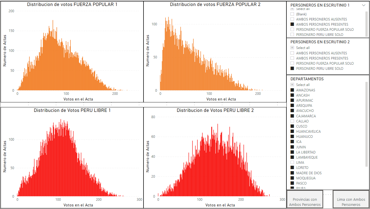
Figura Resumen: En Regiones sin Lima, la distribución de votos de Fuerza Popular no es consistente. Como lo muestra la siguiente figura, la distribución muestra forma normal cuando ambos personeros están presente (1), pero cuando únicamente el personero de Perú Libre está presente (2), la curva es extremadamente sesgada. Lo que no es consistente para la misma población regional, que muestra resultados diferentes cuando se segrega usando la variable de personeros presentes durante el escrutinio. El mismo patrón se muestra en detalle en varios departamentos. 

Introducción

En las elecciones presidenciales Peruanas de la segunda vuelta 2021, se puede visualizar que la distribución estadística de los votos de Fuerza Popular, muestra distorsiones con una distribución muy sesgada con un número alto de mesas con votación muy baja para Fuerza Popular.

La ubicación geográfica (departamento, provincia, distrito, local) sería la única variable que explicaría estas distorsiones como producto de un fenómeno regional, donde la votación de Fuerza Popular resulta en un alto número de mesas con muy bajas votaciones en favor de Fuerza Popular.

El análisis presentado en este documento incluye una nueva variable: la información de los personeros que participaron en el escrutinio.

Las actas de cada mesa contienen secciones donde firman los miembros de mesa y los personeros presentes durante la instalación, escrutinio y sufragio de cada mesa.

Para este análisis se procesó y contabilizó la data de personeros durante el escrutinio de más de 85,816 mesas, que son más del 99% del total de las mesas que se habilitaron en las elecciones. Se pueden determinar cuatro casos diferentes para cada mesa:

  1. Ambos personeros de Fuerza Popular y Perú Libre estuvieron presentes durante el escrutinio.
  2. Únicamente estuvo presente el personero de Fuerza Popular durante el escrutinio.
  3. Únicamente estuvo presente el personero de Perú Libre durante el escrutinio.
  4. Ningún personero estuvo presente durante el escrutinio.

Total de personeros

Esta información revela patrones en los datos que no pudieron ser identificados previamente con la data publicada por la ONPE.

En la figura 1, se puede ver que Perú Libre pudo cubrir más de 36,149 mesas con sus personeros, mientras Fuerza popular solo pudo cubrir alrededor de 29,235 mesas con sus personeros durante el escrutinio de los votos.

También se observa que el número de mesas donde únicamente estuvo el personero de Perú Libre y no estuvo el de Fuerza Popular, fueron alrededor de 11,210 mesas. El número de mesas donde solo estuvo el personero de Fuerza Popular y no estuvo presente el personero de Perú Libre, fueron 4,296 mesas, en otras palabras Perú Libre tuvo más del doble de mesas cubiertas únicamente por un personero de un partido.

Hubo cerca de 24,939 mesas a nivel nacional, donde ambos personeros, de Perú Libre y Fuerza Popular, estuvieron presentes durante el escrutinio. Y finalmente, hubo 45,398 mesas donde no estuvieron presentes ambos personeros.

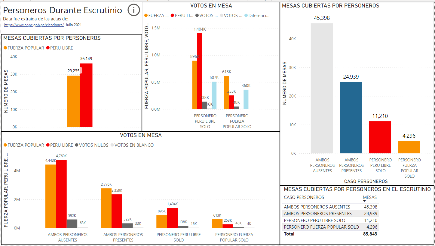
Figura 1: Personeros Durante el escrutinio

Distribución Normal

La curva de campana, mostrada en la figura 2, es el tipo de distribución para una variable que se considerada normal o Gaussiana.

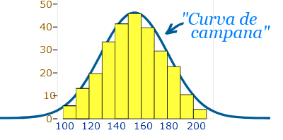
Figura 2: Curva Normal o de Gauss

Distribución de Votos a Nivel Nacional

A nivel nacional, la distribución total de los votos de Fuerza Popular no presenta una forma de curva de campana o curva normal, como se ve en la figura 3, mientras que la curva de distribución de votos de Perú Libre a nivel nacional, si presenta una forma de campana o forma de curva normal.

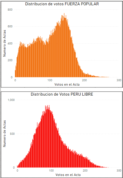
Figura 3: Distribución a nivel nacional de los votos en las mesas para las elecciones de segunda vuelta en Perú 2021. La curva de Fuerza Popular no es normal, mientras que la curva de Perú Libre si muestra una curva normal o gaussiana.

Lima versus Regiones sin Lima: Curva Normal versus curva Sesgada

En la Figura 4, se muestra la distribución de los votos de Fuerza Popular en Lima y en regiones sin Lima. Se puede identificar que en Lima y Callao la curva es normal, mientras que en Perú-sin Lima, la distribución de votos esta sesgada a la izquierda donde hay una cantidad grande de actas con votos muy bajos a favor de Fuerza Popular.

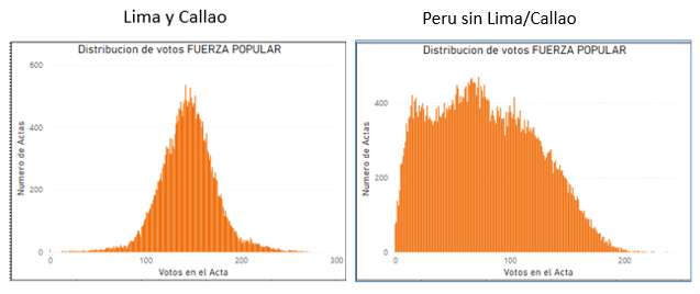
Figura 4: Comparación de la distribución de votos de Fuerza Popular en Lima/Callao versus las otras regiones del Perú sin Lima. La curva de Lima/Callao es definitivamente normal y la curva del Perú sin Lima presenta distorsiones.

Una explicación de este resultado propone que la población en ciertas regiones votó en forma diferente a Lima y esto resulto en una cantidad alta de mesas con votos muy bajos para Fuerza Popular.

Distribución en la región Lima es Normal

En la figura 5, se puede apreciar que en Lima la curva es normal para toda la región Lima/Callao y que seleccionando los casos donde los dos personeros estuvieron presentes, la curva también tiene una forma normal, lo que es consistente con la región geográfica de Lima y Callao.

Cuando ambos personeros están presente durante el escrutinio, el resultado de la votación es más fiable y exacta, ya que hay balances y chequeos de ambos personeros, razón por la que usamos este caso de personeros para poder comparar con los resultados totales en cada región.

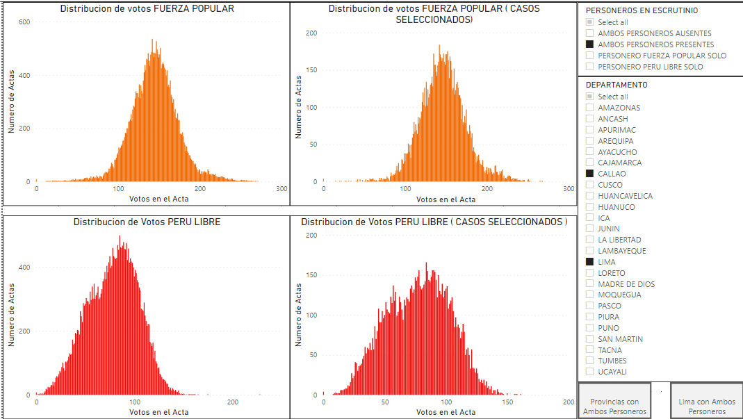
Figura 5: LIMA/CALLAO: Comparación de la distribución de votos en Lima versus la distribución de votos en Lima con solo mesas donde ambos personeros están presentes durante el escrutinio. Las curvas son consistentes en la región, sin importar que los personeros de ambos partidos estuvieran presentes durante el escrutinio.

Conflicto en la Distribución en regiones fuera de Lima: curva es sesgada y normal en la misma región

El patrón de curva sesgada es el que se esperaría en las regiones de Perú-sin Lima. Si se selecciona solo las mesas en departamentos del Perú-sin Lima, donde ambos personeros están presentes, se esperaría obtener la misma curva este sesgada a la izquierda, para que sea consistente con el comportamiento de la población de la misma región geográfica.

En la figura 6, se comparan las distribuciones de votos de las mesas en regiones del Perú-sin Lima. En el lado izquierdo se muestra la curva de todas las mesas de votos de Fuerza Popular en Perú-sin Lima, en el cual se nota que esta curva esta sesgada hacia la izquierda. En el lado derecho de la figura, se ha seleccionado solo las mesas donde los dos personeros de los dos partidos estuvieron presente en las mesas de Perú-sin Lima. En este caso, la curva ya no está sesgada y se convierte en una curva normal, que es opuesto a resultado de las regiones que tienen una curva sesgada a la izquierda.

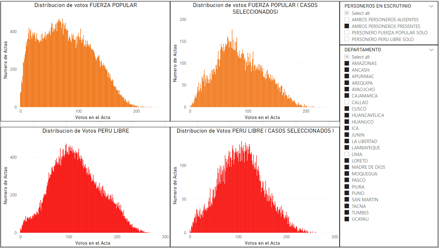
Figura 6: DEPARTAMENTOS EXCLUYE LIMA/CALLAO. Comparación de la distribución de votos en departamentos fuera de la capital versus la distribución de votos de la misma región con las mesas donde ambos personeros estuvieron presentes durante el escrutinio. Las curvas de votos de Fuerza Popular esta sesgada a la izquierda y cuando se seleccionan solo las mesas con ambos personeros presentes durante el escrutinio, la curva es peculiarmente normal. El comportamiento no es consistente en la región.

Las dos curvas de Fuerza Popular de la figura 6 no son consistentes con la ubicación geográfica de Perú-sin Lima, porque son diferentes dependiendo de la variable de personeros presentes durante el escrutinio.

En la figura 7, cuando se selecciona y compara con las mesas donde solo hubo personeros de Perú Libre se ve evidentemente un resultado muy diferente, para Perú-sin Lima. La curva extremadamente segada a la izquierda, que evidencia baja votación para Fuerza Popular.

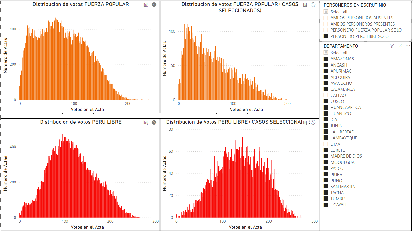
Figura 7: Comparación de la distribución de votos en regiones sin Lima versus la distribución de votos en las mismas regiones sin Lima con solo las mesas donde solo estuvo el personero de Perú Libre presente durante el escrutinio. Los votos de Fuerza Popular están sesgados a la izquierda cuando solo está presente el personero de Perú Libre.

Distribución en los Departamentos

Teniendo un resultado no consistente en regiones fuera de Lima, donde la curva total es sesgada, pero es normal cuando los dos personeros están presentes, el siguiente paso es comparar las mismas curvas a nivel de departamento.

En la figura 8, se puede observar las curvas a nivel de cada departamento y en especial en los departamentos que se señalan con un recuadro rojo: Cusco, Cajamarca, Puno y otros muestra un sesgo pronunciado a la izquierda.

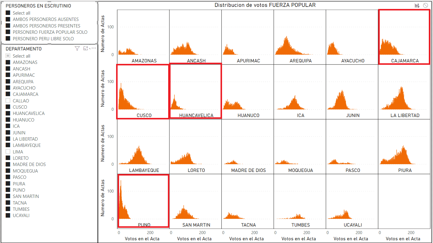
Figura 8: Distribución de votos de Fuerza Popular de cada departamento. Muestra varios departamentos con curvas sesgadas a la izquierda.

En la figura 9, cuando se selecciona solo las mesas donde están presentes ambos personeros, las curvas tienden a ser normales, tal como se ve en el agregado de las regiones. Note la diferencia de los departamentos de Cajamarca, Cusco y Puno con formal normal con la de la figura 8, donde los mismos departamentos muestran una curva de votos sesgadas.

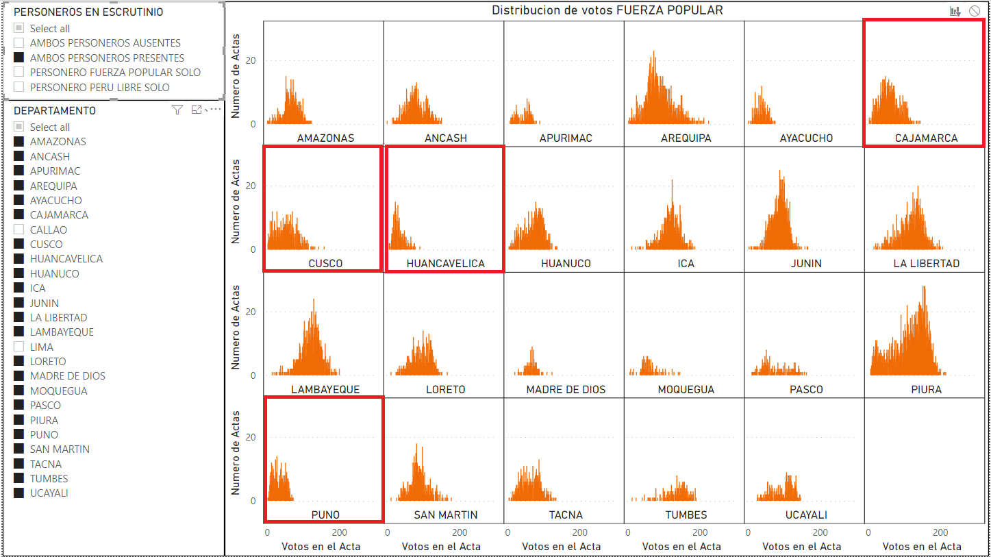
Figura 9: Distribución de votos de Fuerza Popular de cada departamento con mesas donde estuvieron presentes ambos personeros de Fuerza Popular y Perú Libre durante el escrutinio. Las curvas no están sesgadas a la izquierda, las curvas muestran un patrón de curva normal.

Y por último, en la figura 10, cuando se seleccionan solo las mesas donde Perú Libre tuvo un personero y Fuerza Popular no estuvo presente, las curvas se distorsionan notablemente hacia la izquierda que muestra una cantidad elevada de votos bajos para fuerza popular.

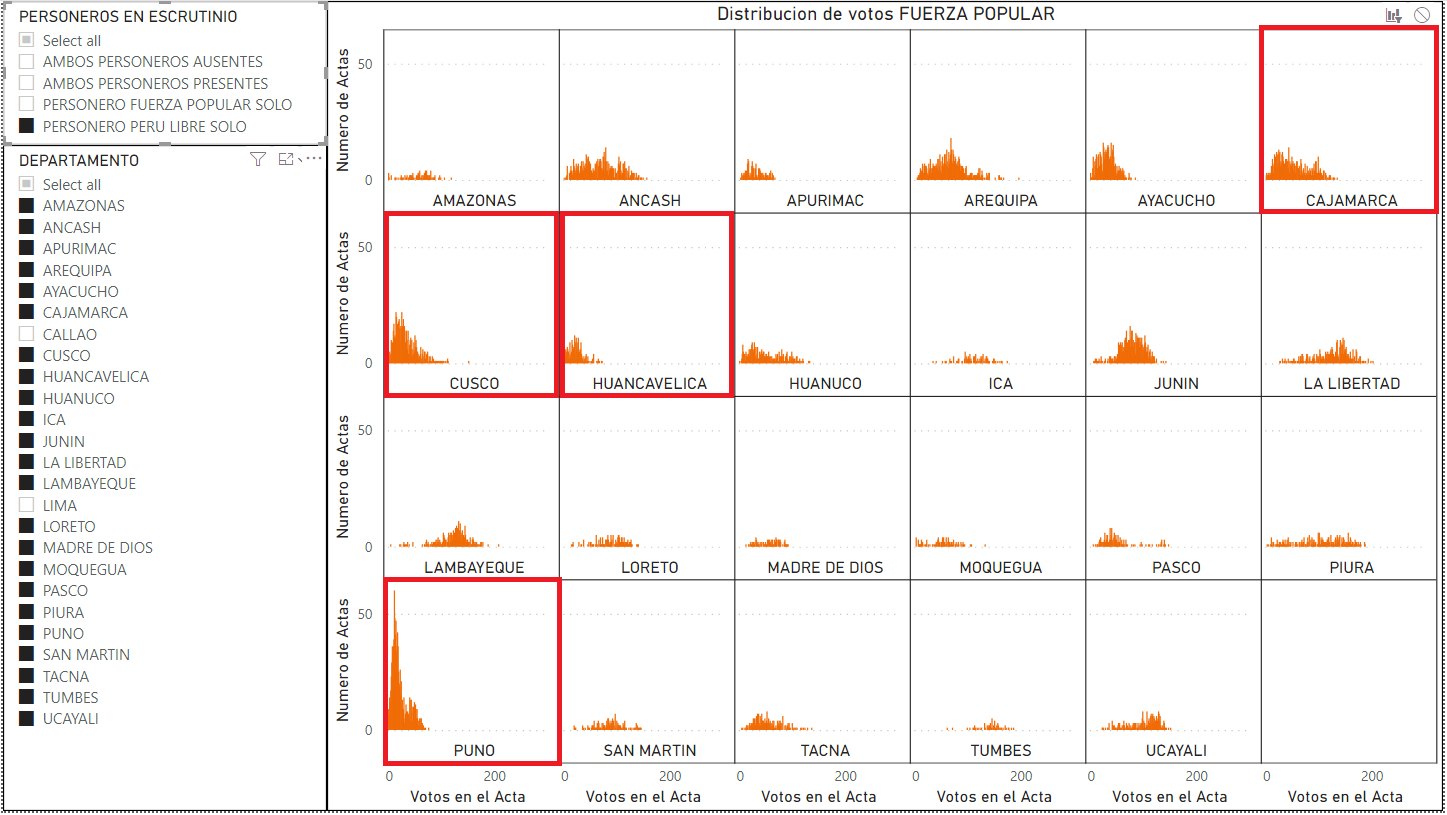
Figura 10: Distribución de votos de Fuerza Popular de cada departamento con mesas donde estuvieron presentes solo personeros de Perú Libre durante el escrutinio. Las curvas muestran un sesgo muy amplio hacia la izquierda.

Caso cuando no hay personeros en la mesa

El caso cuando no hay personeros de ningún partido en la mesa durante el escrutinio debería ser examinado con cuidado. En el entrenamiento a personeros de Perú Libre se recomendó a sus seguidores a ser miembros de las mesas donde les tocaba sufragar, tal como lo dice en el documento de entrenamiento de Perú Libre en la Figura 11.

Si este fuera el caso, el impacto de las distorsiones incluiría también los casos donde no hubo personeros durante el escrutinio de las mesas, pero podría haber influencia escondida de seguidores de Perú Libre como miembros de mesa, sin personeros en mesa.

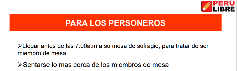
Figura 11: Documento Oficial de capacitación de personeros de Perú Libre.

Publicado en Abril de 2021 en la página web oficial de Perú Libre:

http://perulibre.pe/wp-content/uploads/2021/04/capacitacion-personeros.pdf

Impacto en los resultados finales

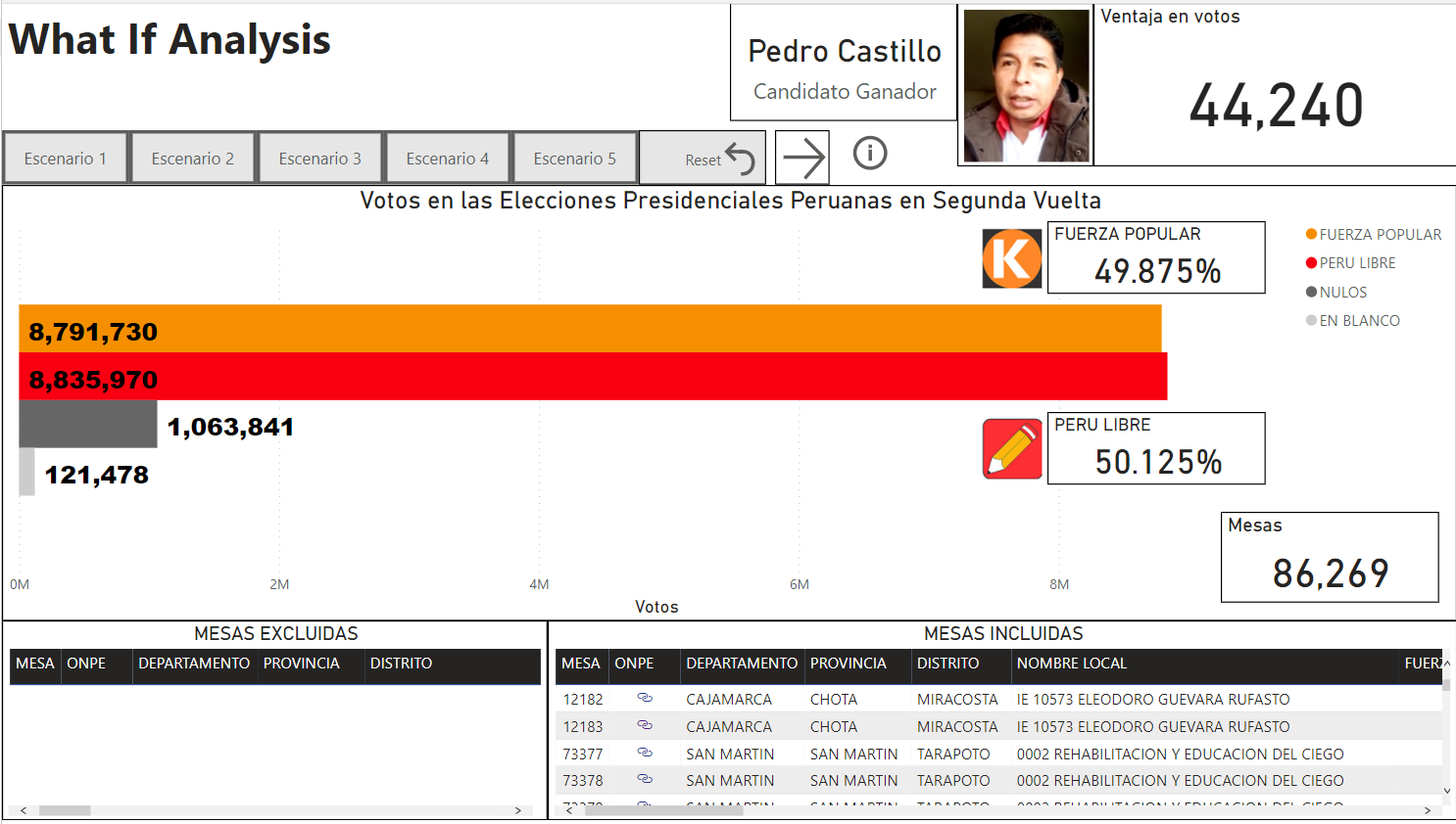
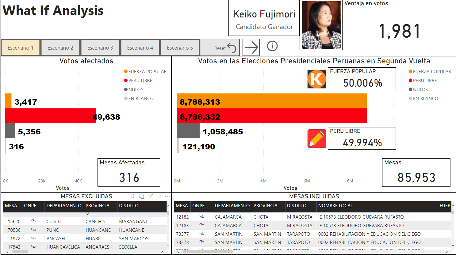
El impacto de los personeros fue muy determinante en las elecciones de segunda vuelta en número total de votos. En la figura 12, se puede ver el resultado de la simulación de un escenario donde se cuentan las mesas que tuvieron dos personeros de ambos partidos: Perú Libre y Fuerza Popular o ningún personero en mesa, eliminando las mesas donde solo un personero de un partido está presente. Fuerza Popular obtiene una ventaja de 103,657 votos. Lo que resulta en una diferencia de más de 147,897 votos si se agrega la diferencia de 44,240 votos a favor de Perú Libre. Esto demuestra que el factor personeros es importante y determinante para el resultado final de las elecciones a nivel nacional.

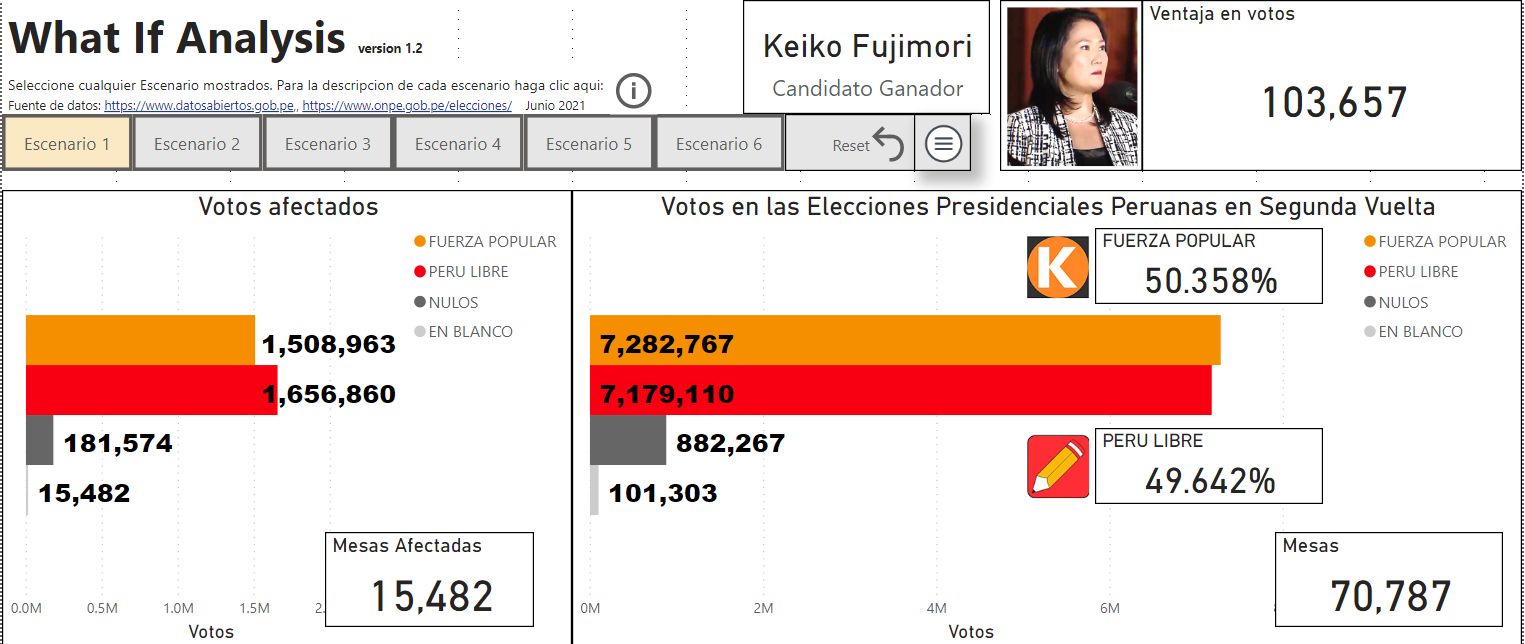
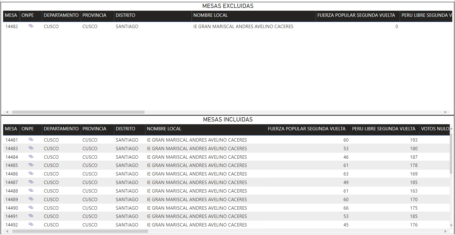
Figura 12: Escenario donde se eliminan las mesas donde personeros de Perú Libre estuvieron únicamente en la mesa y se eliminan las mesas donde los personeros de Fuerza Popular estuvieron únicamente en la mesa.

Conclusion

Con esta nueva información se abren preguntas acerca de las regiones sin incluir Lima/Callao:

¿Por qué los votos a favor de Fuerza Popular no son consistentes dentro de cada región?

¿Por qué las curvas son diferentes cuando se comparan los votos en los casos que hay dos personeros presentes versus cuando únicamente está el personero de Perú Libre presente dentro de cada región?

La curva de votos a favor de Fuerza Popular es sesgada en algunas regiones. Pero la curva no es sesgada cuando se toma en cuenta mesas donde ambos personeros están presentes durante el escrutinio en la misma región.

Cual otra variable, fuera de la de personeros, podría explicar este patrón irregular de resultados de las votaciones cuando esta el personero de Perú Libre?

Estos datos encontrados, rechazarían la hipótesis que la distribución de los votos de Fuerza Popular en regiones al interior del país esta sesgada debida solo a que la población en estas regiones tiene un patrón de votación diferente. Este análisis de los datos de los personeros, evidencia resultados en la votación diferente o inconsistente para la misma población regional, cuando ambos personeros están presentes y cuando solo el personero de Perú Libre está presente. Los resultados de la votación no son consistentes para el mismo departamento o en la misma región. Dependiendo del caso de personeros presentes, la curva es sesgada y en el otro caso la curva es normal.

La variable de personeros durante escrutinio explica este sesgado mejor que la variable geográfica y es finalmente la que determina el resultado final de los votos de Fuerza Popular. Estas distorsiones o sesgado a nivel regional se agregan y resultan en distorsiones a nivel nacional.

Como se muestra en el análisis de escenarios, estas distorsiones tienen un impacto determinante en el resultado final se las elecciones. Lo que resultaría, en caso de eliminar casos de mesas con personeros únicos de ambos partidos, en una ventaja a favor de fuerza popular de 103,657 votos.

Por esto hace necesario hacer una investigación más amplia, tomando en cuenta los casos expuestos para determinar la validez de los resultados.

Categories
Datawarehouse Power BI

What-If Analysis for 2021 Peruvian Presidential Elections

The Interactive report was published here:  https://bit.ly/2SxBY4H

The following is an overview series of data analysis using different tools of the data resulting from the latest 2021 Peruvian Presidential Elections. The Left-wing candidate Pedro Castillo, received 50.125% against 49.875% for the Right-wing candidate, Keiko Fujimori.

The “Fuerza Popular” party’s candidate, Keiko Fujimori, is calling for an audit after alleging “grave irregularities”.

Many of these irregularities are being challenged and resolved by electoral authorities that can lead to having votes annulled in the polling stations.

In this analysis, we try to point out the magnitude or impact of some irregularities and figure out if these cases are isolated or if they are significant in number of votes that could affect the final outcome.

The Dataset

Two datasets were published by Peruvian official authorities corresponding to first and second round of the elections.

Resultados por mesa de las Elecciones Presidenciales 2021 Primera Vuelta – [Oficina Nacional de Procesos Electorales (ONPE)

https://www.datosabiertos.gob.pe/dataset/resultados-por-mesa-de-las-elecciones-presidenciales-2021-primera-vuelta-oficina-nacional-de

Resultados por mesa de las Elecciones Presidenciales 2021 Segunda Vuelta – [Oficina Nacional de Procesos Electorales (ONPE)

https://www.datosabiertos.gob.pe/dataset/resultados-por-mesa-de-las-elecciones-presidenciales-2021-segunda-vuelta-oficina-nacional-de

The first round participated “Fuerza Popular” and “Peru Libre” among other 16 parties from right, center and left wing.

The most granular level of data in these datasets are called “mesas” or “actas”, which are the pooling stations where the votes are record. Each “acta” has a maximum of 300 people registered to vote.

It is very important to familiarize with the dataset before any analysis. There are some records that should not be part of the counting because they are null out already by Electoral Peruvian Authorities as the ones with “ESTADO ACTA” field where the value “ANULADA”, which means that the record has been null out with zeroes due to irregularities.

Atypical Results in Pooling Stations covered by these Scenarios

Under Peruvian law, if the irregularity of an “acta” is demonstrated, the electoral authority should null the “acta” and all the votes would zero out for both candidates.

The scenarios are described in detail within the report. While we have specified five different scenarios, there may be more scenarios that can lead the same results.

Each scenario shows an atypical or peculiar pattern that once is detected, then is removed from the counting for both parties to have fair effect across the voting which affect both candidates using the same criteria.

Some scenarios test the variances between votes in the first round and the second round and qualify as peculiar some extreme cases where the vote of one party reduces dramatically when compare to the voted from the first round. Other scenarios use number of votes resulting in the pool goes to zero or one.

These scenarios can be tuned using parameters live votes, variation of votes and variation of votes in percentages.

The result of each scenario is shown in the chart, where we can see the impact of the exclusion of votes in both parties.

We can drill through details at the locality level, where we can observe the “mesas” excluded from the counting due to anomaly filter out by the scenario.

We can see the detail at the “mesa” or “acta” level. In the sample below we can see the distortion of votes in one single “acta”. All right wing votes obtained in the first round disappeared in the second round.

Tools

Tools used are MS SQL Server and Python for data processing and Power BI for data analysis.

Next

In some following articles we’ll use other techniques used in election forensics try to determine if the results are statistically normal or statistically abnormal:

  • Testing the correlation between vote share of a party and turnout.
  • Checking if the votes received by a candidate obey Benfords’s law
  • Checking for disproportionate presence of 0s in the “actas”.
  • Deviation from statistical laws observed in election data.
  • Using machine learning algorithms to detect anomalies.
Categories
Datawarehouse Power BI SSAS

“Power BI for Large Databases with Composite Mode” at South Florida Power BI User Group

Power BI for Large Databases with new Composite Mode presentation by Hector Villafuerte at the South Florida Power BI User Group.

Today’s enterprise business analytics requires run complex analytic queries against large datasets stored in different sources like Azure SQL Database, Azure Analysis Services, Azure SQL Data Warehouse, Apache Hive, Apache Spark. In this session, BI Architect and Microsoft Certified Professional, Hector Villafuerte focuses upon the design, architecture and best practices that allows Power BI to offer the best functionality and performance combination. Throughout the session, we explore various large datasets and witness how to implement Power BI and different data technologies to achieve high performance and visual capabilities.

DATE: Thursday – October 4th, 2018
TIME: 6:00 pm

– ADDRESS:
Nova Southeastern University
Main Campus – Davie
3301 College Avenue
Davie, FL 33314

Categories
Datawarehouse Power BI SSAS

My presentation for SQLSATURDAY 755 South Florida Conference

This is the presentation for my session at SQL Saturday, South Florida, June 9 2018

Link to download PPT: Download Presentation

Categories
Datawarehouse

SQL Server 2016 On-Premise with Row-Level Security with Active Directory (Part II)

In the previous article, I introduced a simple way to implement Row-Level-Security implementation for Microsoft SQL Server 2016 database with Active Directory.

Here, I’ll show you a more efficient way to implement RLS when you deal with millions of records in your database and thousands of users in your active directory.

Below is the original implementation of a RLS security predicate:

CREATE FUNCTION RLS.GeographyAccessPredicate(@GeographyKey AS INT)

RETURNS TABLE

WITH SCHEMABINDING

AS

RETURN SELECT 1 AS AccessResult

FROM dbo.DimGeography G

WHERE

G.GeographyKey = @GeographyKey AND

(

(

G.CountryRegionCode = 'US' AND IS_MEMBER('DOMAIN\AW United States') = 1

)

OR

(

G.CountryRegionCode = 'GB' AND IS_MEMBER('DOMAIN\AW United Kingdom') = 1

)

OR

(

G.CountryRegionCode = 'DE' AND IS_MEMBER('DOMAIN\AW Germany') = 1

)

OR

(

G.CountryRegionCode = 'FR' AND IS_MEMBER('DOMAIN\AW France') = 1

)

OR

(

G.CountryRegionCode = 'CA' AND IS_MEMBER('DOMAIN\AW Canada') = 1

)

OR

(

G.CountryRegionCode = 'AU' AND IS_MEMBER('DOMAIN\AW Australia') = 1

)

)

There are two performance issues in this filter predicate. First, there is a WHERE condition that slows down the query performance. The GeographyAccessPredicate function contains OR conditions for each country, which it will denied the use of indexes in the tables.

Second, we use a function called IS_MEMBER, which evaluate whether the current user is a member of the specified Active Directory group. This function will execute poorly when we query tables with millions of rows and we have thousands of active directory users and groups in our domain.

In order to improve the performance, instead of calling IS_MEMBER function, I’m going to create a table in the database to keep Active Directory users and groups. This Active Directory user and group table will allow me to join the data with the table and remove the function IS_MEMBER from the security policy predicate. It will simplify and improve the performance of the query execution.

CREATE TABLE [dbo].[DimActiveDirectoryUser](

[LoginName] [varchar](50) NOT NULL,

[GroupName] [varchar](150) NOT NULL,

CONSTRAINT [PK_DimActiveDirectoryUser] PRIMARY KEY CLUSTERED

(

[LoginName] ASC,

[GroupName] ASC

)WITH (PAD_INDEX = OFF, STATISTICS_NORECOMPUTE = OFF, IGNORE_DUP_KEY = OFF, ALLOW_ROW_LOCKS = ON, ALLOW_PAGE_LOCKS = ON) ON [PRIMARY]

) ON [PRIMARY]

In order to populate this table, we can execute a Power Shell script or create a ADSI linked server. In this article, I’ll use ADSI linked server:

USE [master]

GO

EXEC master.dbo.sp_addlinkedserver @server = N'ADSI', @srvproduct=N'Active Directory Service Interfaces', @provider=N'ADSDSOObject', @datasrc=N'adsdatasource'

EXEC master.dbo.sp_addlinkedsrvlogin @rmtsrvname=N'ADSI',@useself=N'False',@locallogin=NULL,@rmtuser=N'domain\YourUser',@rmtpassword='Your Password'

GO

EXEC master.dbo.sp_serveroption @server=N'ADSI', @optname=N'collation compatible', @optvalue=N'false'

GO

EXEC master.dbo.sp_serveroption @server=N'ADSI', @optname=N'data access', @optvalue=N'true'

GO

EXEC master.dbo.sp_serveroption @server=N'ADSI', @optname=N'dist', @optvalue=N'false'

GO

EXEC master.dbo.sp_serveroption @server=N'ADSI', @optname=N'pub', @optvalue=N'false'

GO

EXEC master.dbo.sp_serveroption @server=N'ADSI', @optname=N'rpc', @optvalue=N'false'

GO

EXEC master.dbo.sp_serveroption @server=N'ADSI', @optname=N'rpc out', @optvalue=N'false'

GO

EXEC master.dbo.sp_serveroption @server=N'ADSI', @optname=N'sub', @optvalue=N'false'

GO

EXEC master.dbo.sp_serveroption @server=N'ADSI', @optname=N'connect timeout', @optvalue=N'0'

GO

EXEC master.dbo.sp_serveroption @server=N'ADSI', @optname=N'collation name', @optvalue=null

GO

EXEC master.dbo.sp_serveroption @server=N'ADSI', @optname=N'lazy schema validation', @optvalue=N'false'

GO

EXEC master.dbo.sp_serveroption @server=N'ADSI', @optname=N'query timeout', @optvalue=N'0'

GO

EXEC master.dbo.sp_serveroption @server=N'ADSI', @optname=N'use remote collation', @optvalue=N'true'

GO

EXEC master.dbo.sp_serveroption @server=N'ADSI', @optname=N'remote proc transaction promotion', @optvalue=N'true'

GO


Be sure to replace the values for the following parameters @rmtuser=N’domain\YourUser’,@rmtpassword=’Your Password’.

The following is the script used to synchronize our active directory with the new table DimActiveDirectoryUser in the AdventureWorks database. Notice that I only synchronize the groups that start with the wildcard: “AW*”, since they are the only groups used in my application.

USE AdventureWorksDW2014

GO

TRUNCATE TABLE DimActiveDirectoryUser

GO

DECLARE @GroupName VARCHAR(50)

DECLARE db_cursor CURSOR FOR

SELECT CN

FROM OpenQuery(ADSI,

'SELECT cn, ADsPath FROM ''LDAP://DC=domain,DC=com'' WHERE objectCategory=''group'' AND cn=''AW*'''

)

OPEN db_cursor

FETCH NEXT FROM db_cursor INTO @GroupName

WHILE @@FETCH_STATUS = 0

BEGIN

DECLARE @OPENQUERY nvarchar(4000), @TSQL nvarchar(4000), @LinkedServer nvarchar(4000)

SET @LinkedServer = 'ADSI'

SET @OPENQUERY = 'INSERT INTO DimActiveDirectoryUser(LoginName, GroupName) '

SET @OPENQUERY = @OPENQUERY + ' SELECT sAMAccountName, ''' + @GroupName + ''' FROM OPENQUERY('+ @LinkedServer + ','''

--SET @OPENQUERY = 'SELECT sAMAccountName as Login, CN as Name, GivenName as FirstName,SN as LastName, DisplayName as FullName, UserAccountControl FROM OPENQUERY('+ @LinkedServer + ','''

SET @TSQL = 'SELECT sAMAccountname,givenname,sn,displayname,useraccountcontrol,CN, department FROM ''''LDAP://domain.com/DC=domain,DC=com'''''

SET @TSQL = @TSQL + ' WHERE objectCategory=''''person'''' '

SET @TSQL = @TSQL + ' AND objectClass=''''user'''''

SET @TSQL = @TSQL + ' AND memberOf=''''CN=' + @GroupName + ',OU=AdventureWorks,DC=domain,DC=com'''' '

SET @TSQL = @TSQL + ' '')'

PRINT @TSQL

EXEC (@OPENQUERY+@TSQL)

PRINT @TSQL

FETCH NEXT FROM db_cursor INTO @GroupName

END

CLOSE db_cursor

DEALLOCATE db_cursor

GO

-- Update values to Match Predicate Conditions

UPDATE DimActiveDirectoryUser SET LoginName = 'DOMAIN\' + LoginName, GroupName = REPLACE(GroupName,'AW ','')


Notice that the last update to the LoginName and GroupName facilitates a better match in our security predicate.

Finally, the security predicate is simplified. No more OR conditions or IS_MEMBER function in the security predicate. GeographyAccessPredicate is a join between the DimGeography and the DimActiveDirectoryUser tables.

DROP SECURITY POLICY RLS.AWSecurityPolicy

go

DROP FUNCTION RLS.GeographyAccessPredicate

go

CREATE FUNCTION RLS.GeographyAccessPredicate(@GeographyKey AS INT)

RETURNS TABLE

WITH SCHEMABINDING

AS

RETURN SELECT 1 AS AccessResult

FROM dbo.DimGeography G

INNER JOIN dbo.DimActiveDirectoryUser U

ON G.GeographyKey = @GeographyKey AND

U.LoginName = SUSER_NAME()

AND G.EnglishCountryRegionName = U.GroupName

GO

CREATE SECURITY POLICY RLS.AWSecurityPolicy

ADD FILTER PREDICATE RLS.GeographyAccessPredicate(GeographyKey) ON dbo.DimCustomer

The performance was improved 2X compared with initial version of the security predicate. You’ll notice this difference when dealing with millions of records and thousand users in your active directory. It also depends of the SQL Server configuration.

The following is the query execution plan with the RLS security.

-- Show Plan with Security

ALTER SECURITY POLICY RLS.AWSecurityPolicy WITH (STATE=ON)

GO

SET SHOWPLAN_ALL ON

GO

SELECT COUNT(*) FROM DimCustomer

GO

SET SHOWPLAN_ALL OFF

When implementing RLS keep in mind that there is always an overhead in performance when querying a secured table with RLS. The performance of the queries results depends on how you implement the WHERE condition logic and this logic can be optimized using indexes in the joined fields and avoiding complex functions in your RLS security policy.

Categories
Datawarehouse

SQL Server 2016 On-Premise with Row-Level Security with Active Directory (Part I)

In this article, I’ll explain a basic use case of Row-Level-Security implementation for Microsoft SQL Server 2016 database.

The AdventureWorks Database supports a fictitious, multinational manufacturing company called Adventure Works Cycles. This company sells products around the world. Sales are ordered from five different countries like Unites States, Germany, United Kingdom, Canada, France and Australia.

Adventure Works Cycles has Sales Teams in each of these countries. These teams should only access to data from their corresponding country.

In the picture below, we can see that Ginger Howell, a sales representative from the United States Sales Team, is trying to get information from the Customer Dimension table (Dim Customer).

When GHowell send the query: “SELECT * FROM DimCustomer” to the database. The DimCustomer table contains customer records not only from USA, but from other countries. The database should retrieve to GHowell only the records corresponding to United States Customers.

SQL Server 2016 introduced a new feature the database engine: Row-Level-Security. Row Level Security (RLS) is a concept that provides security at the table row level within the database layer, instead of at the application layer. RLS is accomplished by using a function (predicate) and the security policy that should be implemented by a database administrator.

We are going to use Adventure Works Database as a sample. You can download the database from this link: https://msftdbprodsamples.codeplex.com/releases/view/125550

Download and restore the Adventure Works DW 2014 Full Database Backup.zip

The following is a simplified diagram that includes only three tables from the Adventure Works database: DimCustomer, DimGeography and FactInternetSales

Now, we have Active directory groups corresponding to each country’s sales team.

We create a SQL Login for each of these Active Directory groups.

With the SQL Logins created, we can implement our security policy.

First, we create a new schema, just to keep SQL objects separate from the existing objects.

CREATE SCHEMA RLS

We create the function that we’ll use as a filter predicate for the security policy.

The predicate function is an inline table valued function. This function returns 1 when a row in the DimGeography table matches the corresponding CountryRegionCode (G.CountryRegionCode = ‘US’) and the user executing the query belongs to the corresponding Active Directory group (IS_MEMBER(‘DOMAIN\AW United States’) = 1).

CREATE FUNCTION RLS.GeographyAccessPredicate(@GeographyKey AS INT)

RETURNS TABLE

WITH SCHEMABINDING

AS

RETURN SELECT 1 AS AccessResult

FROM dbo.DimGeography G

WHERE

G.GeographyKey = @GeographyKey AND

(
 (
    G.CountryRegionCode = 'US' AND IS_MEMBER('DOMAIN\AW United States') = 1

  )
  OR

 (
    G.CountryRegionCode = 'GB' AND IS_MEMBER('DOMAIN\AW United Kingdom') = 1
 )
  OR
 (
     G.CountryRegionCode = 'DE' AND IS_MEMBER('DOMAIN\AW Germany') = 1
 )
  OR
  (
     G.CountryRegionCode = 'FR' AND IS_MEMBER('DOMAIN\AW France') = 1
   )
  OR
   (
     G.CountryRegionCode = 'CA' AND IS_MEMBER('DOMAIN\AW Canada') = 1
   )
  OR
  (
    G.CountryRegionCode = 'AU' AND IS_MEMBER('DOMAIN\AW Australia') = 1
  )
)
 

Finally, we add the function as filter predicate on the DimCustomer table:

CREATE SECURITY POLICY RLS.AWSecurityPolicy

ADD FILTER PREDICATE RLS.GeographyAccessPredicate(GeographyKey) ON dbo.DimCustomer

After this our Row-Level-Security is implemented!

Now, we’ll test it by running some scripts. We impersonate a user, GHowell, which belongs to the United States Active Directory.

EXECUTE AS LOGIN = 'DOMAIN\GHowell' -- United States Group

SELECT SUSER_NAME()

SELECT FirstName, LastName, EnglishCountryRegionName

FROM dbo.DimCustomer C

INNER JOIN dbo.DimGeography G

ON C.GeographyKey = G.GeographyKey

The query returns only customers from United States region as expected.

Execute the Revert command to return the execution context back to your user.

REVERT;

Now let’s see what happens behind scenes when the query is executed.

-- Show Plan without Security
GRANT SHOWPLAN TO [DOMAIN\Administrator]
GO
ALTER SECURITY POLICY RLS.AWSecurityPolicy WITH (STATE=OFF)
GO
SET SHOWPLAN_ALL ON
GO
SELECT COUNT(*) FROM DimCustomer
GO
SET SHOWPLAN_ALL OFF

The execution plan shows a simple scan to the DimCustomer table, when the security policy is off.

Now, let’s see how is the execution plan when the security policy is applied.

-- Show Plan with Security

ALTER SECURITY POLICY RLS.AWSecurityPolicy WITH (STATE=ON)
GO
SET SHOWPLAN_ALL ON
GO
SELECT COUNT(*) FROM DimCustomer
GO
SET SHOWPLAN_ALL OFF

When the security policy applied, the execution plan shows an extra join. The filter predicate is being applied and joined to the DimCustomer table.

There is an overhead when Row-Level-Security is applied. This impact in the performance of the queries is affected by the implementation of the filter predicate function.

In our filter predicate function GeographyAccessPredicate, there is a WHERE condition that slows down the query performance. The GeographyAccessPredicate function contains OR conditions for each country, which it will denied the use of indexes in the tables.

Second, we use the function called IS_MEMBER, which evaluate whether the current user is a member of the specified Active Directory group. This also will execute poorly when we query tables with millions rows.

In the next article, I will show a better approach for the predicate function, to speed up the query performance.

Categories
Datawarehouse Power BI

SQL Saturday Presentation – Data Security with Power BI, SSAS, SQL Server and Active Directory

Hector Villafuerte speaking on SQL Saturday South Florida

Saturday, Jun 10, 2017 Conference

http://hectorv.com/wp-content/uploads/sites/3/2017/06/RLS-SQL-Saturday-1.pptx

Bitnami